Custom Cost Matrix

In this example, we cover an interesting feature of assigning user-defined travel costs of traveling from one point to another. NextBillion.ai’s Route Optimization Flexible API would then use these custom costs to arrange the job fulfillment in a way such that the overall costs are minimum.

It is important to highlight that user-defined costs are unitless and they are treated at face value for all calculations. So, without further ado let’s start building an example to understand this powerful feature.

Get Started

Readers would need a valid NextBillion API key to try this example out. If you don’t have one, please contact us to get your API key now!

Setup

Once you have a valid API Key, you can start setting up the components to be used in this example. Let’s take a look at them below.

Jobs & Shipments

We start by defining 4 jobs. For these jobs we add:

• A unique identifier for each job

• Location indexes for each job

• Specify the schedule of jobs. This is done by adding time windows within which a job must be completed. We have not used any time windows for jobs to ensure that timing constraints don’t take precedence over routing cost constraints. This helps us observe the effect of custom costs in isolation. As a clarification, in case time windows and custom costs are used together, time constraints might override few cost constraints such that the task gets fulfilled. This situation is likely to occur when there are no feasible alternatives available for the optimizer, to assign the given task. Route Optimization Flexible API places a high priority on task fulfillment.

• The actual time taken to complete the jobs once the driver/vehicle is at the job’s location i.e. the service time for each job.

Let’s take a look at how the above properties are configured for the jobs:

1{
2  "jobs": [
3    {
4      "id": 1,
5      "location_index": 0,
6      "service": 180,
7      "pickup": [
8        0
9      ],
10      "time_windows": [
11        [
12          1693382400,
13          1693418400
14        ]
15      ]
16    },
17    {
18      "id": 2,

Vehicles

Next, we add the vehicle that is going to fulfill the jobs within the defined constraints. To describe the vehicle and its properties we add:

• A unique ID for the vehicle

• Vehicle shift time or the time window

• Capacity to denote the amount of load that the vehicle can take

• Start_index to denote the point from where the vehicle would start.

• Costs for all vehicles. We have specified a fixed cost of 1000 for the vehicle.

Again, for the sake of simplicity, we are using only 1 vehicle but rest assured Route Optimization Flexible API is equally efficient for any number of vehicles. Readers are encouraged to add multiple vehicles. Once the vehicle and their properties are defined, the resulting vehicles JSON is:

1  "vehicles": [
2    {
3      "id": 1,
4      "start_index": 4,
5      "capacity": [
6        20
7      ],
8      "costs": {
9        "fixed": 1000
10      },
11      "time_window": [
12        1693382400,
13        1693418400
14      ]
15    }
16  ]
17}
18

Locations

Next, we define the locations object and add all the locations used in the problem along with a valid id. The locations object with all the points used in this example:

1{
2  "locations": {
3    "id": 1,
4    "location": [
5      "34.054927,-118.323726",
6      "34.075525,-118.361588",
7      "34.004364,-118.421170",
8      "34.000215,-118.318803",
9      "34.057106,-118.361326"
10    ]
11  }
12}

Custom Cost Matrix

To define the cost of traveling between the locations involved in the optimization problem, we would define a cost matrix. The values in the matrix do not necessarily have to correspond to the actual journey time or distance data. The matrix values can be computed after taking into account any key metric that reflects the actual "cost" of taking a route in your business scenario.

For this example, we are going to use the following cost matrix of randomly selected values that would act as the costs of traveling between different locations.

The figures used in the example cost matrix above in no way reflect the real driving distance between the locations. For example, the actual distance between Job 1 & Job 3 locations is 16 kms whereas the actual distance between Job 1 & Job 2 is 6 kms only.

Once the matrix values are decided and configured, the resulting cost_matrix JSON is:

1"cost_matrix":[
2[0,250,120,100,140],
3[230,0,110,80,230],
4[270,240,0,210,200],
5[300,190,240,0,290],
6[90,100,240,260,0]
7]

Options

Lastly, we would need to set the travel_cost=customized for our cost_matrix to be effective.

1"options":{
2  "objective":{
3     "travel_cost":"customized"
4  }
5}

Optimization POST Request

Now let’s put all these components together and create the final POST request that we will submit to the optimizer.

1curl --location 'https://api.nextbillion.io/optimization/v2?key=<your_api_key>' \
2--header 'Content-Type: application/json' \
3--data '{
4   "description": "Custom Cost Matrix Example",
5   "jobs": [
6       {
7           "id": 1,
8           "location_index": 0,
9           "service": 180,
10           "pickup":[0],
11           "time_windows": [
12               [
13                   1693382400,1693418400
14               ]
15           ]
16       },
17       {
18           "id": 2,

Optimization POST Response

Once the request is made, we get a unique ID in the API response:

1{
2"id": "ce52afbf0c52acfe5a09b2ac901257de",
3"message": "Optimization job created",
4"status": "Ok"
5}

Optimization GET Request

We take the ID and use the Optimization GET request to retrieve the result. Here is the GET request:

1curl --location 'https://api.nextbillion.io/optimization/v2/result?id=ce52afbf0c52acfe5a09b2ac901257de
2&key=<your_api_key>'

Optimization GET Response

Following is the optimized route plan:

1{
2  "description": "Custom Cost Matrix Example",
3  "result": {
4    "code": 0,
5    "summary": {
6      "cost": 1490,
7      "routes": 1,
8      "unassigned": 0,
9      "service": 570,
10      "duration": 4954,
11      "waiting_time": 0,
12      "priority": 0,
13      "delivery": [
14        0
15      ],
16      "pickup": [
17        0
18      ],

Following is a visual representation of the initial locations of tasks, vehicles and the routes suggested after optimization as per the given constraints.

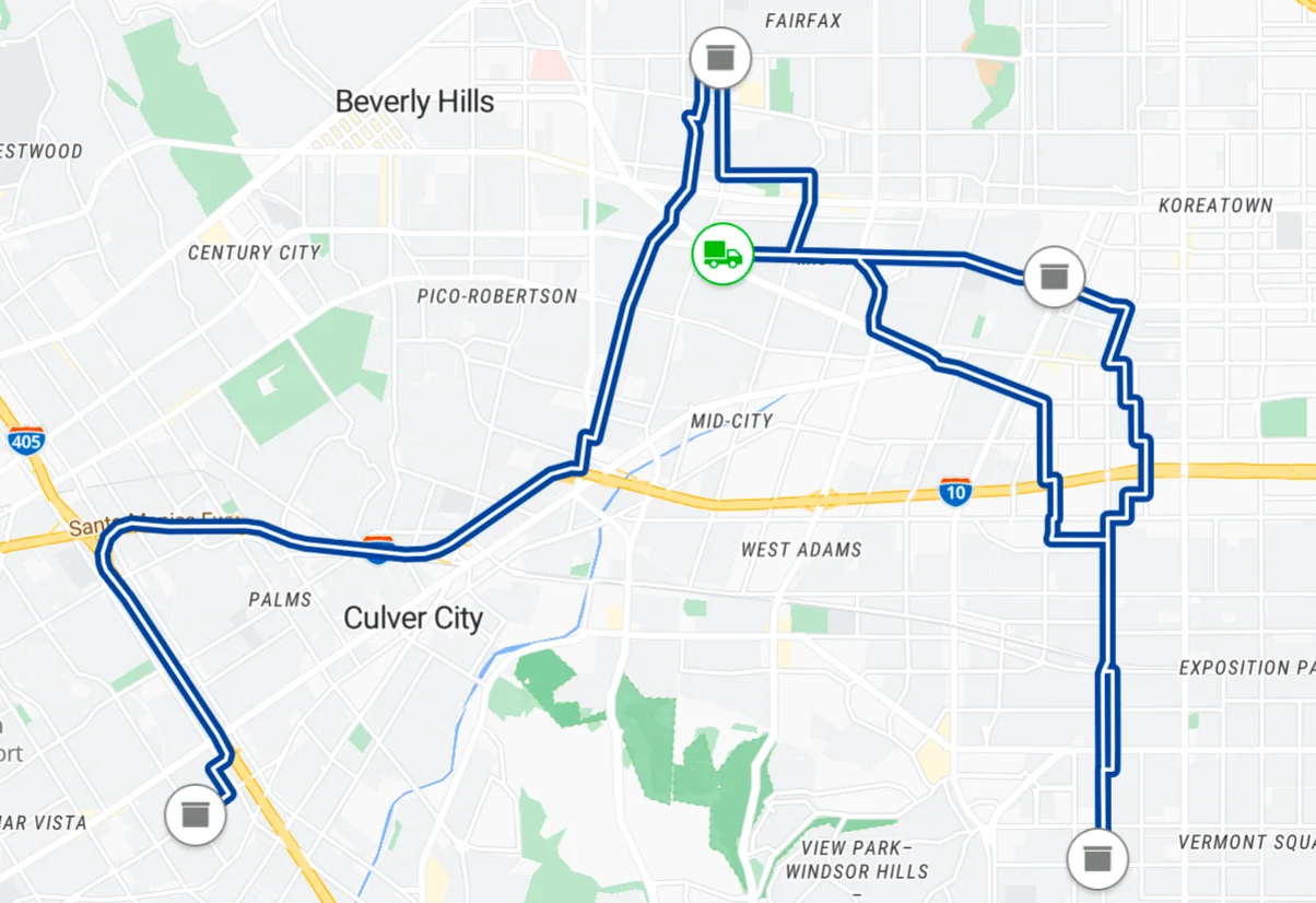
Analyzing the Solution

Looking at the result we can observe some interesting insights:

• We have the regular details of the optimized solution in the summary section. Key detail in context of our example is that none of the jobs remained unassigned.

• In the routes section we can see the details of steps to understand the order in which the jobs were completed.

  • The vehicle, after starting from its start point, completes job 1 first. We can observe from the cost matrix that job 1 was the least costly option indeed from the vehicle's starting point.
  • Once the vehicle completes the job 1, it then goes to job 4 which was most economical (100) among all other valid options, then to job 2 which again was the cheapest option (190) when compared to job 3 which is covered at the last.
  • In order to arrive at the total cost of the optimized solution, 1490, the sum of individual costs of the routes taken (90 + 100 + 190 + 110) is added to the fixed cost of using the vehicle.

As we learned, the custom cost matrix feature of NextBillion.ai’s Route Optimization Flexible API is a powerful way for the users to model real life business constraints. As an experiment, users can try the same example with different cost matrix values or with realistic time windows added to the jobs and find out how these variations affect the original solution.

We hope this example was helpful. Check out some more use cases that Route Optimization Flexible API can handle for you!